Nuclephile Substitution CH3Cl - mMD3
Task
In this example the nucleophile substitution of a Cl- by another Cl- in CH3Cl via meta dynamics is simulated using two collective variables simultaneously.
Input
POSCAR
   1.00000000000000
     9.0000000000000000    0.0000000000000000    0.0000000000000000
     0.0000000000000000    9.0000000000000000    0.0000000000000000
     0.0000000000000000    0.0000000000000000    9.0000000000000000
   C    H    Cl
   1   3   2
Direct
  0.1570348572197245  0.2904054711139102  0.1422643997559632
  0.1466469234176954  0.4066467848992589  0.1077433527138946
  0.0469134772399311  0.2399491465236156  0.1544210764126938
  0.2197893311177821  0.2820094213788985  0.2462070949679763
  0.9809163623144840  0.4723904404063168  0.3674924467383788
  0.2601754409903839  0.1874592103557934  0.9964911656110944
KPOINTS
Automatic
 0
Gamma
 1  1  1
 0. 0. 0.
- For isolated atoms and molecules interactions between periodic images are negligible (in sufficiently large cells) hence no Brillouin zone sampling is necessary.
INCAR
PREC=Low
EDIFF=1e-6
LWAVE=.FALSE.
LCHARG=.FALSE.
NELECT=22
NELMIN=4
LREAL=.FALSE.
ALGO=VeryFast
ISMEAR=-1
SIGMA=0.0516

############################# MD setting #####################################
IBRION=0                                           # MD simulation
NSW=1000                                           # number of steps
POTIM=1                                            # integration step
TEBEG=600                                          # simulation temperature
MDALGO=11                                          # metaDynamics with Andersen thermostat
ANDERSEN_PROB=0.10                                 # collision probability
HILLS_BIN=50                                       # update the time-dependent bias
                                                   # potential every 50 steps
HILLS_H=0.005                                      # height of the Gaussian
HILLS_W=0.05                                       # width of the Gaussian
##############################################################################
ICONST
R 1 5 5
R 1 6 5
- In contrast to the previous examples two collective variables are used simultaneously (and no combination of them).
PENALTYPOT
   5.00000   1.00000   9.00000   0.50000
   5.00000   2.00000   9.00000   0.50000
   5.00000   3.00000   9.00000   0.50000
   5.00000   4.00000   9.00000   0.50000
   5.00000   5.00000   9.00000   0.50000
   1.00000   5.00000   9.00000   0.50000
   2.00000   5.00000   9.00000   0.50000
   3.00000   5.00000   9.00000   0.50000
   4.00000   5.00000   9.00000   0.50000
Calculation
Sometimes it is difficult to find one single parameter that approximates the reaction coordinate well but it is often possible to identify a small set of parameters that form a basis for the reaction coordinate. These parameters (collective variables) can be used in meta dynamics to determine free-energy surface. In this example we use two C-Cl distances as collective variables in the ICONST file. We still want to avoid the dissociation of the vdW complexes, which is an undesired process, hence we define an initial bias potential whose role is to ensure that no C-Cl distance becomes longer than (defined in the PENALTYPOT file).
Running the calculation
The mass for hydrogen in this example is set 3.016 a.u. corresponding to the tritium isotope. This way larger timesteps can be chosen for the MD (note that the free energy is independent of the masses of atoms).
The bias potential is specified in the PENALTYPOT file.
For practical reasons, we split our (presumably long) meta dynamics calculation into shorter runs of length of 1000 fs (NSW=1000; POTIM=1). At the end of each run the HILLSPOT file (containing bias potential generated in previous run) must be copied to the PENALTYPOT file (the input file with bias potential) - this is done automatically in the script run which looks as follows:
#!/bin/bash

runvasp="mpirun -np x executable_path"

# ensure that this sequence of MD runs is reproducible
cp POSCAR.init POSCAR
cp INCAR.init INCAR
rseed="RANDOM_SEED =         311137787                0                0"
echo $rseed >> INCAR


i=1
while [ $i -le 100 ]
do

  # start vasp
  $runvasp

  # ensure that this sequence of MD runs is reproducible
  rseed=$(grep RANDOM_SEED REPORT |tail -1)
  cp INCAR.init INCAR
  echo $rseed >> INCAR

  # use bias potential generated in previous mMD run
  cp HILLSPOT PENALTYPOT

  # use the last configuration generated in the previous
  # run as initial configuration for the next run
  cp CONTCAR POSCAR

  # backup some important files
  cp REPORT REPORT.$i
  cp vasprun.xml vasprun.xml.$i

  let i=i+1
done
- The user has to adjust the runvasp variable, which holds the command for the executable command.
- Please run this script by typing:
bash ./run
Time evolution of distance
During the simulation, the time evolution of collective variable can be monitored using the script timeEv.sh:
#!/bin/bash

rm timeEvol1.dat timeEvol2.dat

i=1
while [ $i -le 1000 ]
do
  if test -f REPORT.$i
  then
    grep fic REPORT.$i |awk '{if (NR%2==1) {print $2} }' >>timeEvol1.dat
    grep fic REPORT.$i |awk '{if (NR%2==0) {print $2} }' >>timeEvol2.dat
  fi
  let i=i+1
done
To execute this script type:
bash ./timeEv.sh
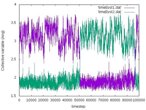
This script creates two files timeEvol1.dat and timeEvol2.dat, which hold the time evolution of the C-Cl distances for both Cl atoms. To visualize that file execute the following command:
gnuplot -e "set terminal jpeg; set xlabel 'timestep'; set ylabel 'Collective variable (Ang)'; set style data lines; plot 'timeEvol1.dat', 'timeEvol2.dat'" > timeEvol.jpg
The obtained time evolution of the collective variables should look like the following:
From this plot we very nicely see that at the beginning the two collective variables run parallel to each other, staying at the same side at approximately the same distance from the centre atom. After approximately 50000 steps the two collective variables cross and switch. This indicates very nicely that the substitution reaction occured. One should note that the atoms come close to each other but never touch each other because of the repulsive forces. So the distances will be of course never 0 but some finite positive distances. After almost 50000 steps the collective variables switch back again. In principle one should obtain that the substitution reaction will go forth and back as the bias potentials are added to potential energy (as already explained in the previous example).
2D free-energy profile
To calculate the free-energy profile in 2D we use the script calcprofile2D.py attached with this example:
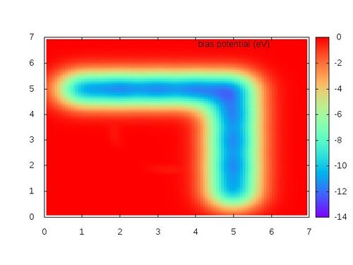
This script projects a set of two-dimmensional Gaussians defined in the input file (such as PENALTYPOT or HILLSPOT) onto a regular 2D grid of points defined by the user. The user is asked to provide the following data: (a) the name of the input file, (b) the initial (x1_min) and final (x1_max) grid points, and the number of grid points (M) for the axis corresponding to the first collective variable, and (c) the initial (x2_min) and final (x2_max) grid points and the number of grid points (N) for the axis corresponding to the second collective variable. The result is written to a file with extension .xyz and it can be visualized by regular plotting tools like Gnuplot.
In our example we will use the following inputs:
Run script:
python calcprofile2D.py
File name?
PENALTYPOT
x1_min x1_max M:
0 7 100
x2_min x2_max N:
0 7 100
The following script (plot_2D_profile.gp) can be used to plot the 2D density:
set terminal jpeg

set palette rgb 33,13,10

set view 0,0

set contour
set noclabel
set pm3d implicit at b
set nosurface

set pm3d map

set cntrparam levels incremental 0., 0.02, 0.5

set out "PENALTYPOT.jpg"
splot "PENALTYPOT.xyz" with lines  title 'bias potential (eV)'
Please execute this script with the following command:
gnuplot plot_2D_profile.gp
The resulting free energy profile should look like the following:


