XANES in Diamond: Difference between revisions
(improve language of step 1 & 2) |
No edit summary |
||
| Line 102: | Line 102: | ||
=== Step 3 Running Calculation === | === Step 3 Running Calculation === | ||
Both the SCF calculation with the core-hole and the subsequent calculation of the dielectric matrix (spectrum) are done in a run of VASP. To minimize the spurious interaction between core-holes in neighboring cells requires large super cells and to reduce the computational time it is advisable to run a parallel VASP calculation | |||
mpirun -np $np vasp_version | |||
Here, ''$np'' corresponds to the number of processes and the ''_version'' in the executable stands for ''std'', ''gam'', and ''ncl'': the standard, <math>\Gamma</math>-point only, and non-collinear version, respectively. | |||
The <math>3\times3\times3</math> cell used in this tutorial gives qualitatively correct results and can be completed even with a small number of processes. You can verify the spectrum on the larger <math>4\times4\times4</math> cell, which we provide in the tar file of this tutorial. | |||
=== Step 4 Extraction of XAS Spectrum === | === Step 4 Extraction of XAS Spectrum === | ||
The XAS spectrum is the imaginary part of the frequency-dependent dielectric function, which is written in the {{TAG|OUTCAR}} file | |||
frequency dependent IMAGINARY DIELECTRIC FUNCTION (independent particle, no local field effects) density-density | frequency dependent IMAGINARY DIELECTRIC FUNCTION (independent particle, no local field effects) density-density | ||
E(ev) X Y Z XY YZ ZX | E(ev) X Y Z XY YZ ZX | ||
| Line 117: | Line 118: | ||
... | ... | ||
Usually we are interested in the sum of all components of the dielectric matrix. You can | Usually we are interested in the sum of all components of the dielectric matrix. You can obtain this by the script provided in this tutorial | ||
perl ./plot_core_imdiel.pl | |||
which will create the file CORE_DIELECTRIC_IMAG.dat containing the sum of the imaginary part of the dielectric matrix. | |||
We compare the results obtained with VASP to experimental<ref name="Ma.PRL"/> and theoretical<ref name="Tallefumier.PRB"/> XAS spectra from literature provided in the files ''C_XAS_aligned_to_VASP.dat'' and ''C_PARATEC_aligned_to_VASP.dat'', respectively. The theoretical reference calculation was obtained using the PARATEC code and relies on PAW/Pseudopotential similar to VASP. Both spectra are shifted to coincide with the VASP at the first peak. We provide a script with this tutorial to compare these literature results to the spectrum obtained with VASP | |||
gnuplot gnuplot.script | |||
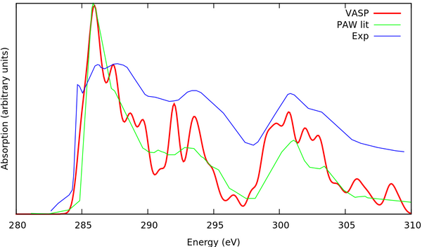
The file ''plot.sh'' constitutes a convenient wrapper around these post processing steps. The resulting spectra should look like this:<br /> | |||
[[File:Fig XAS 4.png|600px]] | [[File:Fig XAS 4.png|600px]] | ||
Note that the absolute values of the experimental peak positions is not captured due to fundamental limitations of local DFT. Usually there is even a noticeable deviation between calculations using different codes. However, the relative position of the peak and their intensity can be experimental offset of the spectrum (absolute value of the first peak) is rather impossible to reproduce, since the calculated core energies are very different compared to experiment. It is accepted in literature to look at the relative peak positions in the spectra and the spectra can be scaled arbitrarily . In this example we scaled the experiment to VASP, since in this way the obtained results can be very easily compared to the experiment using a script. Usually one would either scale the first peak to 0 or would scale the calculated value to the experiment. Additionally the intensity of the spectrum can be scaled arbitrarily. So in this example we align the position and the height of the first peak for the calculations. The experiment is a little bit more tricky. It's a matter of taste what to consider as the first peak, but we decided that most likely the second peak corresponds to the first peak in the calculations and the first peak in experiment is a shoulder that is simply not pronounced in experiment. | |||
Another important issue is the broadening. Many factors contribute to the experimental broadening depending totally on the experimental setup and hence it is impossible to reproduce the broadening exactly. We can choose a broadening that gives approximately the same width as experiment, but the choice of broadening parameters is rather arbitrary than systematic. For simplicity in this example we choose to use a 0.5 eV constant Lorentzian broadening (this is the only type of broadening built in for the calculation of XAS spectra in VASP). For more elaborate spectra we strongly advise users to choose a 0.05 eV broadening and apply the desired broadening in post-processing. | Another important issue is the broadening. Many factors contribute to the experimental broadening depending totally on the experimental setup and hence it is impossible to reproduce the broadening exactly. We can choose a broadening that gives approximately the same width as experiment, but the choice of broadening parameters is rather arbitrary than systematic. For simplicity in this example we choose to use a 0.5 eV constant Lorentzian broadening (this is the only type of broadening built in for the calculation of XAS spectra in VASP). For more elaborate spectra we strongly advise users to choose a 0.05 eV broadening and apply the desired broadening in post-processing. | ||
Revision as of 15:05, 7 December 2018
(UNDER CONSTRUCTION)
Important: This feature will be only available from VASP 6.0.
Task
Calculation of the XANES K-edge in diamond using the supercell core-hole method.
Input
POSCAR
cubic diamond
 3.567
0.5 0.5 0.0
0.0 0.5 0.5
0.5 0.0 0.5
 2
direct
0.0 0.0 0.0
0.25 0.25 0.25
Above, we show the POSCAR file for the primitive unit cell of diamond. Note that we will not use this structure as input for the calculation. Instead, we use it to construct a POSCAR file for a super cell actually used in the calculation.
INCAR
System = DIAMOND
ALGO = FAST
ISMEAR = 0; SIGMA = 0.1;
ICORELEVEL = 2
CLNT = 1
CLN = 1
CLL = 0
CLZ = 1.0
CH_LSPEC = .TRUE.
CH_SIGMA = 0.5
NBANDS = 300
LREAL = A
- To promote a core electron into the conduction bands and hence create the core-hole ICORELEVEL=2 has to be set. This corresponds to the final state approximation.
- CLNT=1 selects the first atom species in the POSCAR file.
- CLN=1 selects main quantum number 1 (hence K-edge).
- CLL=0 selects angular quantum number 0 (s).
- CLZ=1.0 selects the charge of the core hole. By setting this number to a fractional value we can mimic different screenings of the electrons. These non-integer values should only be used with caution, since this purely exploits error cancellation and does not correspond to a physically correct description of the screening.
- By setting CH_LSPEC=.TRUE., we enable the calculation of matrix elements between core and conduction states and the calculation of the core electron absorption spectrum.
- The broadening of the core electron absorption spectrum is controlled by the tag CH_SIGMA. Usually it is good practice to set this value low and broaden the spectrum in post processing.
- We have to set NBANDS to a larger value to consider enough conduction band states in the calculation.
- Since super cells are used the calculation of the projection operators in real space (LREAL=A) is much faster.
Calculation
Step 1 build a supercell
In the periodic boundary conditions of VASP, the core-hole interacts with its periodic replica so that we need sufficiently large super cells to reduce this spurious interaction. To this end, we employ successively larger cells until the spectrum shows no significant changes. For this tutorial, we illustrate the calculation of a core-hole using a cell to allow for a reasonably fast calculation. However, for converged values one should use at least super cell.
The super cell can be obtained by either taking the file POSCAR.3x3x3 provided with this tutorial or constructing the POSCAR file from the primitive cell using p4vasp, which is demonstrated below:
- Open p4vasp by typing p4v on the terminal.
- Load the primitive cell by clicking on File→Load system:
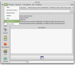
- Multiply cell in each direction (enter 3 for each direction) by clicking on Edit→Multiply Cell:
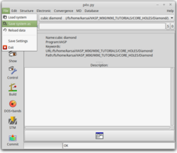
- Save new system by clicking on File→Save system as:
Step 2 Prepare input files
The first few lines of the generated POSCAR file for the super cell should look like the following
cubic diamond
3.567
 +1.5000000000  +1.5000000000  +0.0000000000
 +0.0000000000  +1.5000000000  +1.5000000000
 +1.5000000000  +0.0000000000  +1.5000000000
 54
Cartesian
 +0.0000000000  +0.0000000000  +0.0000000000
 +0.2500000000  +0.2500000000  +0.2500000000
 +0.5000000000  +0.0000000000  +0.5000000000
 ...
Here, all the 54 atoms are of the same species (line 6). To distinguish between the atom with the core-hole and the rest, we treat one atom as a different species. Choosing the first atom, we replace the 54 in the 6th line with 1 and 53 and obtain the following POSCAR file
cubic diamond
3.567
 +1.5000000000  +1.5000000000  +0.0000000000
 +0.0000000000  +1.5000000000  +1.5000000000
 +1.5000000000  +0.0000000000  +1.5000000000
 1 53
Cartesian
 +0.0000000000  +0.0000000000  +0.0000000000
 +0.2500000000  +0.2500000000  +0.2500000000
 +0.5000000000  +0.0000000000  +0.5000000000
 ...
In the INCAR file, we specify that the first species carries the core-hole by setting CLNT=1. We create a POTCAR file with the PAW/PS information for both species. Since both species are carbon this amounts simply to the concatenation of the POTCAR file for carbon
cat POT_C POT_C > POTCAR
We provide the resulting POTCAR file for this core-hole calculation in the tar file of this tutorial.
To calculate accurate spectra, we need to include a sufficient number of conduction states. The required number of bands depends on the number of electrons in the system and the energy range of the spectrum. We can manually adjust the number of bands with the NBANDS variable. However, since the computation time increases drastically with the number of bands, selecting initially very large numbers is also not advisable. Hence, one has to increase the number of bands to find the optimum of computational effort and accuracy. In this tutorial, we use NBANDS=300.
The other input variables in the INCAR file are described above.
Mind: The multiplicity of the species carrying the core-hole has to be 1 otherwise the code will not work. Also mind that the selected species (CLNT in the INCAR file) is consistent with the order of the species specified in the POSCAR and POTCAR files.
Step 3 Running Calculation
Both the SCF calculation with the core-hole and the subsequent calculation of the dielectric matrix (spectrum) are done in a run of VASP. To minimize the spurious interaction between core-holes in neighboring cells requires large super cells and to reduce the computational time it is advisable to run a parallel VASP calculation
mpirun -np $np vasp_version
Here, $np corresponds to the number of processes and the _version in the executable stands for std, gam, and ncl: the standard, -point only, and non-collinear version, respectively. The cell used in this tutorial gives qualitatively correct results and can be completed even with a small number of processes. You can verify the spectrum on the larger cell, which we provide in the tar file of this tutorial.
Step 4 Extraction of XAS Spectrum
The XAS spectrum is the imaginary part of the frequency-dependent dielectric function, which is written in the OUTCAR file
  frequency dependent IMAGINARY DIELECTRIC FUNCTION (independent particle, no local field effects) density-density
     E(ev)      X         Y         Z        XY        YZ        ZX
  --------------------------------------------------------------------------------------------------------------
  243.589609    0.000000    0.000000    0.000000    0.000000    0.000000    0.000000
  243.677325    0.000000    0.000000    0.000000    0.000000    0.000000    0.000000
  243.765042    0.000000    0.000000    0.000000    0.000000    0.000000    0.000000
  ...
Usually we are interested in the sum of all components of the dielectric matrix. You can obtain this by the script provided in this tutorial
perl ./plot_core_imdiel.pl
which will create the file CORE_DIELECTRIC_IMAG.dat containing the sum of the imaginary part of the dielectric matrix.
We compare the results obtained with VASP to experimental[1] and theoretical[2] XAS spectra from literature provided in the files C_XAS_aligned_to_VASP.dat and C_PARATEC_aligned_to_VASP.dat, respectively. The theoretical reference calculation was obtained using the PARATEC code and relies on PAW/Pseudopotential similar to VASP. Both spectra are shifted to coincide with the VASP at the first peak. We provide a script with this tutorial to compare these literature results to the spectrum obtained with VASP
gnuplot gnuplot.script
The file plot.sh constitutes a convenient wrapper around these post processing steps. The resulting spectra should look like this:

Note that the absolute values of the experimental peak positions is not captured due to fundamental limitations of local DFT. Usually there is even a noticeable deviation between calculations using different codes. However, the relative position of the peak and their intensity can be experimental offset of the spectrum (absolute value of the first peak) is rather impossible to reproduce, since the calculated core energies are very different compared to experiment. It is accepted in literature to look at the relative peak positions in the spectra and the spectra can be scaled arbitrarily . In this example we scaled the experiment to VASP, since in this way the obtained results can be very easily compared to the experiment using a script. Usually one would either scale the first peak to 0 or would scale the calculated value to the experiment. Additionally the intensity of the spectrum can be scaled arbitrarily. So in this example we align the position and the height of the first peak for the calculations. The experiment is a little bit more tricky. It's a matter of taste what to consider as the first peak, but we decided that most likely the second peak corresponds to the first peak in the calculations and the first peak in experiment is a shoulder that is simply not pronounced in experiment.
Another important issue is the broadening. Many factors contribute to the experimental broadening depending totally on the experimental setup and hence it is impossible to reproduce the broadening exactly. We can choose a broadening that gives approximately the same width as experiment, but the choice of broadening parameters is rather arbitrary than systematic. For simplicity in this example we choose to use a 0.5 eV constant Lorentzian broadening (this is the only type of broadening built in for the calculation of XAS spectra in VASP). For more elaborate spectra we strongly advise users to choose a 0.05 eV broadening and apply the desired broadening in post-processing.
Apart from the obviously lower broadening width, we get quite reasonable agreement with theoretical literature calculations. We stress again that we used a cell in this example and that our results with respect to cell size are not fully converged. The interested user can repeat the calculations for the cell, which can be done in complete analogy to the cell (set NBANDS carefully since we have many more atoms in the cell). The files for this example are also given in the tar file.
Download
References
Back to the main page.


