Nuclephile Substitution CH3Cl - mMD2: Difference between revisions
| Line 131: | Line 131: | ||
gnuplot -e "set terminal jpeg; set xlabel 'r(Ang)'; set ylabel 'PCF'; set style data lines; plot 'timeEvol.dat'" > timeEvol.jpg | gnuplot -e "set terminal jpeg; set xlabel 'r(Ang)'; set ylabel 'PCF'; set style data lines; plot 'timeEvol.dat'" > timeEvol.jpg | ||
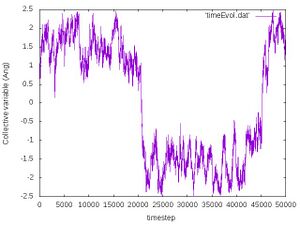
The plot of the collective variable with respect to the timestep should look similar to this: | The plot of the collective variable with respect to the timestep should look similar to this: | ||
[[File:TimeEvol CHCl3 mMD2.jpg|300px]] | [[File:TimeEvol CHCl3 mMD2.jpg|300px]] | ||
Revision as of 10:38, 27 September 2019
Task
In this example the nucleophile substitution of a Cl- by another Cl- in CH3Cl via meta dynamics is correctly simulated by using extra "repulsive potential walls."
Input
POSCAR
   1.00000000000000
     12.0000000000000000    0.0000000000000000    0.0000000000000000
     0.0000000000000000    12.0000000000000000    0.0000000000000000
     0.0000000000000000    0.0000000000000000    12.0000000000000000
   1   3   2
cart
         5.91331371  7.11364924  5.78037960
         5.81982231  8.15982106  5.46969017
         4.92222130  6.65954232  5.88978969
         6.47810398  7.03808479  6.71586385
         4.32824726  8.75151396  7.80743202
         6.84157897  6.18713289  4.46842049
KPOINTS
Automatic
 0
Gamma
 1  1  1
 0. 0. 0.
- For isolated atoms and molecules interactions between periodic images are negligible (in sufficiently large cells) hence no Brillouin zone sampling is necessary.
INCAR
PREC=Low
EDIFF=1e-6
LWAVE=.FALSE.
LCHARG=.FALSE.
NELECT=22
NELMIN=4
LREAL=.FALSE.
ALGO=VeryFast
ISMEAR=-1
SIGMA=0.0516

############################# MD setting #####################################
IBRION=0                                           # MD simulation
NSW=1000                                           # number of steps
POTIM=1                                            # integration step
TEBEG=600                                          # simulation temperature
MDALGO=11                                          # metaDynamics with Andersen thermostat
ANDERSEN_PROB=0.10                                 # collision probability
HILLS_BIN=50                                       # update the time-dependent bias
                                                           # potential every 50 steps
HILLS_H=0.005                                      # height of the Gaussian
HILLS_W=0.05                                       # width of the Gaussian
##############################################################################
- Same INCAR file as in the previous example (Nuclephile Substitution CH3Cl - mMD).
ICONST
R 1 5 0
R 1 6 0
S 1 -1 5
- This file is the same as in the previous example (Nuclephile Substitution CH3Cl - mMD1).
Calculation
In principle, meta dynamics always seeks for the path of least resistance. In the case of our model system this corresponds to the dissociation of the vdW complex (which is linked with a lower barrier than the SN2 reaction). In order to avoid this undesired process, an extra bias potential ("repulsive walls") is used whose role is to restrict our sampling to a relevant region (approx. collective variable ). In fact, the positions of walls can be chosen arbitrarily - we only require that the region between the walls contains all the information we are interested in (in this case we want to see free-energy minima for both "reactant" and "product" as well as the "transition state"). In order for the walls to be effective, we also require that they are significantly higher than the expected reaction barrier (otherwise the likelihood to cross the wall during meta dynamics would be higher than that for the barrier). From the potential energy profile (static calculations not reported here) we obtained a reasonable guess for the reaction barrier - it is about 0.4 eV - hence the height for the wall of 1 eV should be sufficient.
Running the calculation
The mass for hydrogen in this example is set 3.016 a.u. corresponding to the tritium isotope. This way larger timesteps can be chosen for the MD.
The bias potential is specified in the PENALTYPOT file.
For practical reasons, we split our (presumably long) meta dynamics calculation into shorter runs of length of 1000 fs (NSW=1000; POTIM=1). At the end of each run the HILLSPOT file (containing bias potential generated in previous run) must be copied to the PENALTYPOT fiel (the input file with bias potential) - this is done automatically in the script run which looks as follows:
#!/bin/bash

runvasp="mpirun -np x executable_path"

# ensure that this sequence of MD runs is reproducible
cp POSCAR.init POSCAR
cp INCAR.init INCAR
rseed="RANDOM_SEED =         311137787                0                0"
echo $rseed >> INCAR

i=1
while [ $i -le 50 ]
do

  # start vasp
  $runvasp

  # ensure that this sequence of MD runs is reproducible
  rseed=$(grep RANDOM_SEED REPORT |tail -1)
  cp INCAR.init INCAR
  echo $rseed >> INCAR

  # use bias potential generated in previous mMD run
  cp HILLSPOT PENALTYPOT

  # use the last configuration generated in the previous
  # run as initial configuration for the next run
  cp CONTCAR POSCAR

  # backup some important files
  cp REPORT REPORT.$i
  cp vasprun.xml vasprun.xml.$i

  let i=i+1
done
- The user has to adjust the runvasp variable, which holds the command for the executable command.
- Please run this script by typing:
bash ./run
Time evolution of distance
During the simulation, time evolution of collective variable can be monitored using the script timeEv.sh:
#!/bin/bash

rm timeEvol.dat

i=1
while [ $i -le 1000 ]
do
  if test -f REPORT.$i
  then
    grep fic REPORT.$i |awk '{print $2 }' >>timeEvol.dat
  fi
  let i=i+1
done
To execute this script type:
bash ./timeEv.sh
This script creates the file timeEvol.dat. To visualize that file execute the following command:
gnuplot -e "set terminal jpeg; set xlabel 'r(Ang)'; set ylabel 'PCF'; set style data lines; plot 'timeEvol.dat'" > timeEvol.jpg
The plot of the collective variable with respect to the timestep should look similar to this:
If everything goes well, you should observe that the amplitude of oscillations of the collective variable increases (as larger and larger region of configuration space is visited by the meta dynamics) and at some poin the collective variable switches from a positive value (corresponding to reactant) to a negative value (correpsonding to product). At the end of your calculation, you should observe depending on how long you ran the calculation (50 or more ps) one or two crossings of the transition state (where the collective variable is equal to zero).


